|
A Guide to Implementing the Theory of
Constraints (TOC) |
|||||
|
How Can We Characterize Marshalling? There is an inverse to the distribution supply
chain, it’s called marshalling. In
fact, the diagram below is the same one that we used for distribution, turned
on its head, and reworded for log marshalling. Marshalling is a convergent supply chain
from production to end user, and although not as common as a distribution
network it is still critically important to a number of industries. Moreover, many of the same opportunities
that we identified for distribution can also be found in marshalling. Processing of patients in a public health system
should also be a marshalling operation, but currently it isn’t. We will address this in the next page after
examining log marshalling in detail.
Marshalling is characterized by multiple source
nodes which produce a range of products that have some commonality with one
another. Therefore we can obtain the
same type of end product from various combinations of source nodes. The product is then on-sold or moved
through a converging supply chain to an end user. The end user node at the convergence point
is often characterized by “lumpiness” or infrequency (but not necessarily
irregularity) of the operation. A single supply node can’t supply the end user
demand by itself; moreover, the rate at which the end user can consume
product is much greater than the rate at which all the source nodes can
resupply. Therefore there is a
continuous resupply going on to refill the end user node. The other levels in the system don’t manufacture
anything. They may purchase and
on-sell or they may simply reflect storage or a change in mode of
transportation. And although they
don’t have a manufacturing lead time, the do have a resupply lead time. Broadly speaking the resupply lead time can
be characterized as the time taken to load, transport, and unload the
products from one node to another. The time taken between production at the source node
and consumption/purchase at the end user node can be quite considerable –
multiples of months or maybe quarters. If we apply our knowledge of production systems to
supply chains and recognize the current pervasive mode of operation – the
reductionist/local optima approach as we described in the pages on
measurements, people, and process of change – then we could well expect local
efficiency measures to be paramount in marshalling. We can test that by asking ourselves
whether we can in fact currently operate the system in order to have just the
right quantity of just the right material, in just the right place, in good
time – always. If not, then we know
there is room for improvement. Let’s examine a specific case in more detail – log
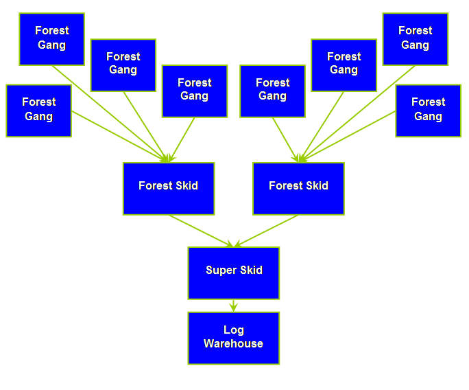
marshalling. The system as drawn above is a generic
representation of a regional export log marshalling operation (regional in a
non-continental sense). The
marshalling chain is an integrated business, harvesting trees, making logs,
and transporting them for sale and pick up by ship. Until the end user has made a purchase and
the logs are loaded onto a ship the system hasn’t made a sale. The system could also be considered as a
local rather than regional log supply system in which case there would also
be aspects of distribution involved.
However the marshalling part would still look very similar we only
need change some of the words, let’s do that.
Log production (growth) has an interesting
characteristic, it doesn’t stop. Trees
continue to grow and mature regardless of whether they are harvested or
not. Plantation trees are grown with a
specific harvest age in mind. Volumes
are large, one arm of the regional diagram for instance currently produces
about 2500 truck & trailer loads of produce a week. Log making and log harvesting are sometimes
combined, and sometimes separate. Log
making has the same properties as a factory node in a manufacturing
system. In fact log making is a small
“V-plant.” We looked briefly at the
characteristics of V-plants in the page on production and again in supply
chain distribution. One of the main
characteristics of V-plants under local optima operation is “stealing,” in
this case issuing cutting orders for one thing but then re-cutting it up to
fulfill something else. As we all know
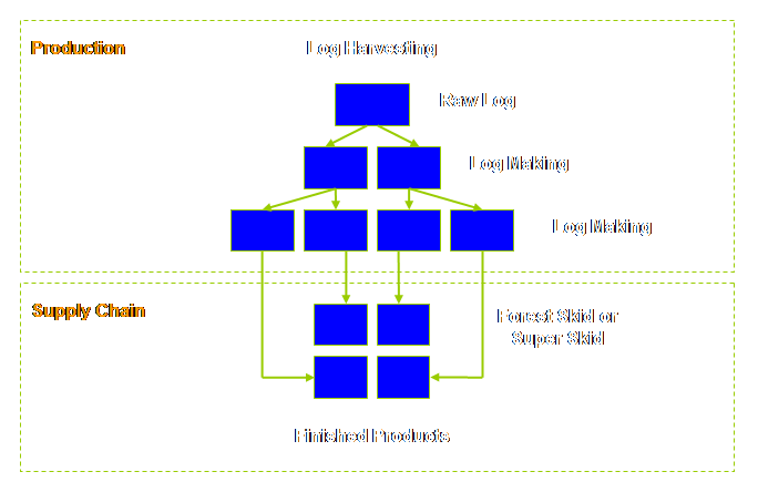
we can re-cut a long log shorter, but we can’t uncut a short log. Let’s draw this V-plant assuming one forest
gang is filling one forest staging node from the diagram above.
In this simple model the raw log goes through a
series of divergent points (class, length, grade). The end product is a range of “finished
goods” stored and awaiting transportation to the next step in the marshalling
supply chain. If the logs were cut to
order, how then could “stealing” be in operation? Quite simply in fact – new orders are
issued to countermand the ones previously issued. The question then arises why are new
cutting orders issued? In New Zealand forest blocks are cut-to-order
(1). For cut-to-order, read
cut-to-forecast, and in this case the forecast horizon is 3-4 months from the
time of cutting to the time of shipping.
Why do we need to cut so far out from final sale? This long lead time arises from the fact that it
takes a lot longer to harvest, transport and pre-position the loads in the
port-side marshalling yards than it does to load-out from the port-side
marshalling yards to the ship. Ships
mostly like to load-out at about the same time – towards the end of the month
and as quickly as possible. The
purchasing company also likes to leave finalizing the shipload until the last
moment. As you can see the problems
are quite similar to distribution, and the solutions, as we will see, are the
similar as well. Currently, then, we might expect that sometimes we
miss maximizing a sale (quantity and grade and size requested) and hence the
return to the owner. In a system which
is not internally constrained by production, failing to maximize a sale should
be a crime. We need a plan of attack. Our plan of attack should be starting to look very
familiar – it’s our 5 step focusing process once again; (1) Identify the system’s constraints. (2) Decide how to Exploit the system’s constraints. (3) Subordinate everything else
to the above decisions. (4) Elevate the system’s constraints. (5) If in the previous steps a constraint has been broken Go back to step 1, but do not allow inertia to cause a
system constraint. In other words; Don’t
Stop. What is the constraint in this system? The limited number of customers who want to
buy product from us. Once again that
almost answers the second question – how to exploit the constraint? We need to ensure that we can always meet
our customer demand and not miss any sales, nor sell something of less value
than the customers’ original desire.
We will need to deduce the mechanism to best exploit the
constraint. We will also need to
develop how to best subordinate the system once the exploitation strategy is
in place. To enable us to determine the exploitation and
subordination tactics we need to examine the properties of log marshalling
networks in a little more detail.
Let’s do that. Let’s take a line item – a grade and size and
quantity of log. What is the accuracy
of the forecast for demand 1 month from shipping? Plus or minus 5% maybe? Sometimes we could sell 105% of the current
demand and sometimes we might sell 95% of current demand. What then is the accuracy of the forecast 2
months from shipping? Plus or minus
10% maybe? Sometimes we could sell
110% of current demand and sometimes we might sell 90% of current
demand. How about 3 months then? Probably the accuracy for a line item 3-4
months out is more like plus or minus 20% percent of current demand. Even if we can determine the aggregate
demand for all line items right on the nail (plus or minus 5%) we will still
have too much of some line items and not enough of some other line items. So, just as in distribution, the accuracy of the
forecast detail degrades with the length of our forecast horizon. The aggregate demand might also alter as
well over longer forecast periods.
There are two unavoidable consequences of this. The first is that we will also have missed
some sales. The second is that will
have some stock that sits on the wharves for several months – stock that was
paid to be cut and transported and which we haven’t yet sold. Logs, however, are a perishable
product. They develop fungal sap
stains within a short period of time.
At that time they become “pulp” logs for pulp and paper production and
are downgraded. Then a prime log has
to be re-transported back down the system for sale at a much, much, lower
margin. This is similar to meeting
your “use-by-date” in distribution and just as expensive in terms of
opportunity lost. Let’s call this suite of problems “forecasting
error.” However, in addition to forecast variation we have
another factor – supply variation.
Supply variation occurs because we try to cut whole blocks according
to some predicted yield of grade and size and quantity that are a best match
to our forecast demand. We can’t cut
half a tree down, and under plantation management regimes we can’t cut 60% of
a block and leave the remainder standing.
Therefore, it isn’t so difficult to produce too much of some items and
not enough of others, regardless of the forecast that we are working to. Therefore we miss sales in two ways; (1) Forecasted demand variation. (2) Actual supply variation. So this is a little different from pure
manufacturing where we do have the option of only making what is required
(but try telling manufactures that; manufacturers like making things
regardless). We end up using valuable capacity to cut trees that
we don’t sell (we guessed that they were the right trees to cut when we cut
them), and then we feel as though we don’t have sufficient capacity to cut
the trees that we are selling. It’s a
bit like the factory source node in distribution, even though the aggregate
sales might be level at retail, the demand level at the factory can be quite
lumpy – and although overall there is sufficient total capacity we don’t have
sufficient peak capacity to handle the induced peaks in demand. To this mix we must add one more component – the
tendency towards local optimization and efficiency measures. In the distribution supply chain we used the analogy
of a V-plant in manufacturing to explain some of the characteristics of
diverging systems. Fortunately because
marshalling is convergent – a big funnel directed at the wharves in the
regional model or the log warehouse in the local model – we don’t quite have
the same problems. For marshalling the
correct analogy from manufacturing is an A-plant. Under traditional management practices in
A-plants the tendency is to misallocate resource time in an attempt to
maximize efficiency and utilization figures.
Large batches are used to keep the measurements high resulting in a
poor component mix and constant shortage of the right parts (2). Furthermore these large batches move in
waves throughout the plant causing temporary bottlenecks to wander from
resource to resource. Since material
is constantly out of balance, overtime is used to ‘catch up’ so that
shipments can be made on time (2). We
can expect similar things to happen in a marshalling supply chain. Unlike distribution where the consumer demand must
be aggregated back to the source node, in marshalling the consumer demand
must be disaggregated back to the source nodes. The effect however is the same, in addition
to forecasting error due to time, we have an error due to improper
disaggregation or allocation, that is to say our predisposition to local
efficiency will cause us to do more log making and making of particular
grades in some places (because it is deemed to be locally efficient) and less
in other places (because it is deemed to be locally inefficient) at any one
time than pure disaggregation of market demand would have required. Let’s call this “allocation error.” Now we can understand better why instructions to
cutting crews change even though we are dealing with long lead times and
steady demand. We have in our supply
chain both multiple dependencies (layer to layer) and considerable room for
variation from; (1) Forecasted demand variation. (2) Actual supply variation. (3) Local efficiency
drivers/allocation error. We can’t do anything about forest supply
variation. In an open market system,
pricing reflects the difference between real supply and real demand. However we certainly can do something about
forecast variation, and we certainly can do something about local efficiency
based drivers. We have been calling the supply chain described here
a marshalling supply chain. However, a
more accurate description would be marshalling and consolidation. Consolidation according to harvesting
production-push. The production-push
is signaled by a forecast about the future based upon recent past trends and
intuition about the near future. This
system is called cut-to-order but in reality it is cut-to-forecast. In the Theory of Constraints manufacturing
application, drum-buffer-rope, we saw how work is pulled through the system
by the constraint schedules. In the
same way just-in-time also pulls work through the system. We need to invoke the same principles here
in our marshalling system; we need a consumer or customer demand-pull. That way we produce a mix that most closely
matches what is required by the system to satisfy demand. However, how can we do this when we have
such long resupply times? Well, what
if we were to consider each layer of nodes in the chain one at a time rather
than the whole chain from beginning to end?
What if we were to consider resupply to just the next level? Then lead times would be much, much,
shorter. Surely that would help. Well, we have already described such a situation in
the previous page on distribution; we have seen how to replenish using
replenishment buffers in such a fixed-frequency supply chain system, so we
really need to invoke the same mechanism here – pull-to-replenish. We are going to move from harvesting production
push-to-forecast to customer demand pull-to replenish. However, before we look at the solution
there is one more aspect to consider. Fortunately this is not a problem that is unique to
forestry it common to all primary and extractive producers. If you remove the milk fat and milk protein
from milk to make cheese you had better have a good market for the milk sugars
that are left behind or a good market for the industrial alcohol that you can
manufacture from the milk sugars. If
you extract the milk fat for butter then you had better have a good market
for the skim milk powder that you can manufacture from the remaining milk. In forestry the yield, the throughput for the whole
tree, determines the yield for the system.
How do we determine the yield?
Well, applying throughput analysis to each product stream would be a
very good start. Essentially we are
interested in the contribution margin that each product stream can yield,
rather than some measure of net profit per product. In other words we are interested in
determining significant variable costs but not in allocating indirect
overhead or direct labor. It is almost
certain that under such analysis the order of sales preference (to maximize
cash inflow) will change. Hard rock gold miners of yesterday and today also
operate a type of marshalling supply chain.
Ore of various grades occurs in various veins and even within the same
veins in different places. The
greatest total yield from the mine comes from ore-grade management. This approach may be viewed as keeping the
high-grade ore diluted with lower grade ore, or keeping the lower grade ore
bulked up with high-grade ore. How do
we extend this to forestry? Basically
we may have to accept some mobility between forest blocks in order to
maintain proper yields – the yields that the market is willing to pay for, or
pay the most for overall. We are
cutting trees to make money after all. We have identified the leverage point; sales to the
customer, and we have identified the exploitation strategy – customer demand
pull-to-replenish, but how do we go about it?
Well, we will use the Theory of Constraints supply chain solution –
replenishment. If you are unfamiliar
with fixed-frequency variable-quantity replenishment then please check the
explanation on the replenishment page – it is important. The demand is determined at each stage in the supply
chain and buffered accordingly. So
where do we start? Probably the best
place to start is the place where the aggregate demand is best known and in a
marshalling system this is at the convergence point, the port-side
marshalling yards in the regional model or the super skid in the local
model. At all it is at his point that
we have the greatest quantity and variety of source material (uncut logs) and
the greatest range of products to fulfill.
What about the next node or nodes up, how do we
treat them? Just the same, the aggregate
buffer size must be sufficient to supply the next node down over the period
of reorder and resupply for that item from the next node up in the
system. As we move back up the system
from port-side to forest staging in the regional model or log warehouse to
forest gang in the local model we must size the buffers needed to ensure
continual supply. We no longer need to
forecast. We may still need to issue
cutting orders – but only to instigate replenishment the forest staging
buffers and no more. Let’s summarize
this. Introducing replenishment buffers and increasing
resupply frequency automatically We have moved the protection for the system to the
best possible area – portside/super skid.
This is the area with greatest aggregate supply and greatest aggregate
demand and in this instance it is also closest to the customer. As we move back up the system and the nodes
become more disaggregated then we run a risk that our safety portion of the
buffer may become too large. However,
we can reduce this impact by increasing the frequency of transportation at
the most critical level (forest staging) to reduce the overall size of the
buffers in the positions between the forest gangs and the first major
consolidation. We may also need to
increase the frequency of issuing cutting orders, and increase the
flexibility for gangs to mill concurrent blocks according to actual yield
demands – as determined by buffer consumption. We previously used forecasting because there was a
considerable time delay between the producer and the consumer – caused in
part by the inventory. Now we can
resupply just to the next node based upon most recent need. The time delay we are dealing with is from
one node to the next, not from the beginning to the end of the process,
therefore we don’t need detailed forecasting anymore. In essence we have synchronized the whole
supply chain by buffering each node against the supply and variation in
supply leading into that node and the demand and variation in demand leading
out of it. In fact each node is a
buffer. In the previous page on distribution we saw how
General Motors had succeeded in replenishing Cadillac dealers in Florida for
a very broad range of popular custom configurations (if you are buying a
Cadillac you get to determine not only body and color, but also engine,
transmission, and numerous other options that on most vehicles are
fixed). In the past it was taking a
dealer 6-10 weeks to pull a replacement car from the factory direct. With replenishment to a regional
distribution center dealers can get a replacement within 24 hours in over 95%
of the time (3, 4). Of course logs are
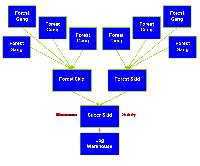
not Cadillacs but the principle remains the same. The potential for replenishment in log
marshalling is considerable. In the regional model the maximum safety is not
located in the forest with individual gangs but rather at the point of
maximum consolidation – the super skid or log plant. Two large-scale local supply chains in New
Zealand use either a log making yard or a log making plant. This is termed a super skid. Another large-scale local supply chain
carries out log making in conjunction with harvesting in the forest. In Europe especially there seems to be a
trend in mechanical harvesting to cut-to-length in the forest. This might be alright for high value small
scale operations but porting it to large-scale commodity plantation forests
does not appear to be an optimal solution. Now that we have identified the constraint (leverage
point) and proposed an exploitation strategy, how do we subordinate the
subsystems in the process to the goal of the overall system? We are really asking; how do we address
deviations from our plan, our plan of attack (5). Deviation from subordination results from; (1) Not
doing what was supposed to
be done for the non-constraints. (2) Doing what was not
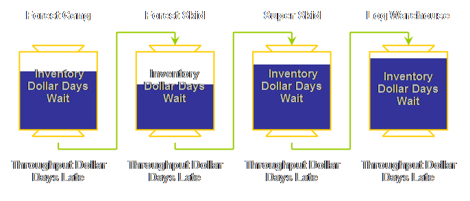
supposed to be done for the non-constraints. Remember the customer is the constraint, so
everything else in the system that is not the customer is a
non-constraint. Goldratt has two
measures that cover the two cases above (5).
One is a measure of lateness which covers not doing what was supposed
to be done, the other is a measure of waiting-in-process which covers doing
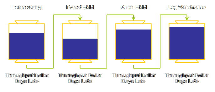
what was not supposed to be done. The measure of lateness is attached to any order at
any node that can’t be filled immediately from stock for a buffer or can’t be
filled by the due date for a cutting order.
If we can’t dispatch sufficient logs of a sufficient grade and size to
fulfill an order to a downstream node, that order is late until dispatched in
full. We calculate its value as the
throughput (sales value at the final point of sale less total variable costs)
multiplied by the days late. Let’s
draw this.
If replace current forecasting with simple
replenishment using buffers we would certainly avoid our current forecasting
error. Therefore, why can’t we just
treat log marshalling as a simple replenishment system through a linear
supply chain of dependent vendors or dependent nodes? Well, it turns out that there are a number
of reasons for this; (1) We must sell the entire tree, all
of the time. (2) We must consolidate from numerous
source nodes. (3) We must currently subordinate the
source nodes to the point of sale. (4) We must position the protection in
the place that best protects the whole system. Of these; positioning the protection for the system
in the place that does the most good is probably the most important; this
mitigates our other major error – allocation error. And the best place for the protection,
unlike distribution, is closest to the customer. In fact, however, in both cases the
protection is a loaded at the point where volumes are most aggregated. In marshalling that happens to be the
port-side marshalling yards in the regional model or the super skid in the
local model. And if we are space
constrained there, then we must move the protection to the next node up and
ensure we have fast and frequent replenishment from that node. Because marshalling deals with a convergent
supply chain it is not a case of simple replenishment. We begin to determine the replenishment buffers for
line items at the point where we know the demand with the greatest degree of
certainty – at the port-side log yards.
The log yards “see” the aggregate demand of the whole system, the
peaks and the toughs smoothed out to the largest extent. Then we work through the individual nodes
in the next layer, and the next layer after that until we reach the point of
origin. We avoid forecasting error. We avoid allocation error. The unavoidable outcome is that we no longer have
too little of the right material in the right place in the right time because
our “plant” capacity (cutting gangs) is now “smoothed” and not wasted making
unnecessary “emergency” jobs. There are two caveats. Firstly some nodes might be space
constrained; then we have to consider moving the safety forward or failing
that back to the next level up and improving transportation
volume/frequency. Secondly, because we
must attempt to drive yield some “by-product (product in excess of market
demand) may occur. We have to accept
in the first instance that market pricing will reflect this, but secondly we
should seek mafia solutions for selling such product at a higher price than
the market currently pays. The counter
argument is that some lines may always be in poor supply and hence yield very
good prices – we won’t complain about this except maybe wish that 25 years
earlier someone had got the figures correct! There are a number of unavoidable outcomes; (1) Increased throughput. (2) Decreased total inventory. (3) Stock-outs are no longer caused by
the supply chain. (4) Over-stock is no longer caused by the
supply chain. (5) Less emergency orders. In fact we should have just the right amount of just
the right material in just the right place – always. If this explanation seems quite simple and
straightforward then that is excellent; then we know that we have developed
an understanding of replenishment as applied to log marshalling. If experience tells us that reality is more
complicated than this generalized case, then that too is excellent. Now we are in a position to better
understand how to apply this methodology to our own particular situations. Marshalling is like its inverse, distribution,
without quite all of the complications of a divergent supply chain. However in the particular case of log marshalling
we must sell the whole tree and this adds an additional dimension to the
problem. Moreover marshalling, like
distribution, is currently served by forecasting. Thus trees are felled and logs are cut
deterministically some time out from final sale. The inevitable consequence is that
sometimes we don’t make enough of the right logs and sometimes we make too
many of the wrong logs. When we make
too many of the wrong logs some may reach their use-by date and have to be
down-graded and re-transported as pulp logs. We can overcome this by using the supply chain
global solution of replenishment and buffer management. In this case each node acts as a buffer for
the next level and we can dispense with forecasting and it associated
errors. Moreover, we automatically
place the system safety in the place where it provides maximal protection –
the port-side marshalling yards or the super skid. Furthermore, by increasing reorder and
resupply frequency we can improve on current service delivery while decreasing
total log inventory. (1) Penfold,
C., (2003) Log making to market or to order.
New Zealand Forest Industries, September, pp 20-22. (2) Stein, R. E., (1994) The next phase of
total quality management: TQM II and the focus on profitability. Marcel Dekker, pg 36. (3) Stern, G., (1995) GM expands its experiment to improve Cadillac's
distribution, cut inefficiency, The Wall Street Journal (February 8th). (4) Stern, G., and Blumenstein, R., (1996) GM
expands plans to speed cars to buyers.
The Wall Street Journal (October 21). (5) Goldratt,
E. M., (1990) The
haystack syndrome: sifting information out of the data ocean. North River Press, pp 144-155. This Webpage Copyright © 2003-2009 by Dr K. J.
Youngman |